Remote Sensing of Vegetation

slide 1

Remote Sensing of Vegetation

Course lecture introducing the use of remote-sensing data for characterizing vegetation — its seasonal growth cycles, spectral signature, and the indices derived to measure it.

Likely answer edit

Opening slide: the lecture is about using remote sensing to study vegetation — both the biology (phenology, canopy structure, chlorophyll) and the instruments and math (bands, indices) that turn reflected light into a measurement.

Course anchor: this is the deck behind the “Crop Phenological Cycles”, “Vegetation Index (VI)”, “NDVI”, and “EVI” key-term bullets on the exam.

slide 2

Lecture objectives

Phenological cycle
Vegetation indices
- Vegetation Index (VI)
- Normalized Difference Vegetation Index (NDVI)
- Enhanced Vegetation Index (EVI)

Likely answer edit

Lecture objectives. Three things to be able to explain by the end of the deck:

Phenological cycle — how a crop or natural vegetation community changes through the year.
What a vegetation index is and why it works (low red + high NIR signature).
The three main VIs — VI/SR, NDVI, EVI — their formulas, ranges, and where each is used.

slide 3

Vegetation indices — topics

What are vegetation indices?
Why do they work?
Band ratios
Emphasis on leaf area index (LAI), % green cover, chlorophyll content, and green biomass.
NDVI: Normalized Difference Vegetation Index
EVI: Enhanced Vegetation Index

Likely answer edit

Topic roadmap for vegetation indices.

What they are — synthetic band-math layers (not measurements).
Why they work — healthy vegetation’s low red / high NIR reflectance makes ratios diagnostic.
What they correlate with — leaf area index (LAI), % green cover, chlorophyll content, green biomass.
Which ones to know — Simple Ratio (first), NDVI (standard), EVI (improved for dense canopies).

slide 4

Phenological cycle characteristics

Phenology — periodic biological phenomena that correlate with annual climatic conditions.

Phenology tells us when remote-sensing data should be collected for a given purpose:

When are crops planted?
When are they harvested?
When do they reach full development?
When have they not yet developed?

Likely answer edit

Phenology is the study of recurring biological events timed to the annual climate cycle (planting, germination, full canopy, senescence, harvest). It matters for remote sensing because the date you image a scene changes what the sensor sees — peak-biomass imagery maximizes vegetation/soil contrast, while off-season imagery helps separate crop types that overlap when green.

Know: why phenology drives acquisition timing; example cycle for a familiar crop.

slide 5 (picture)

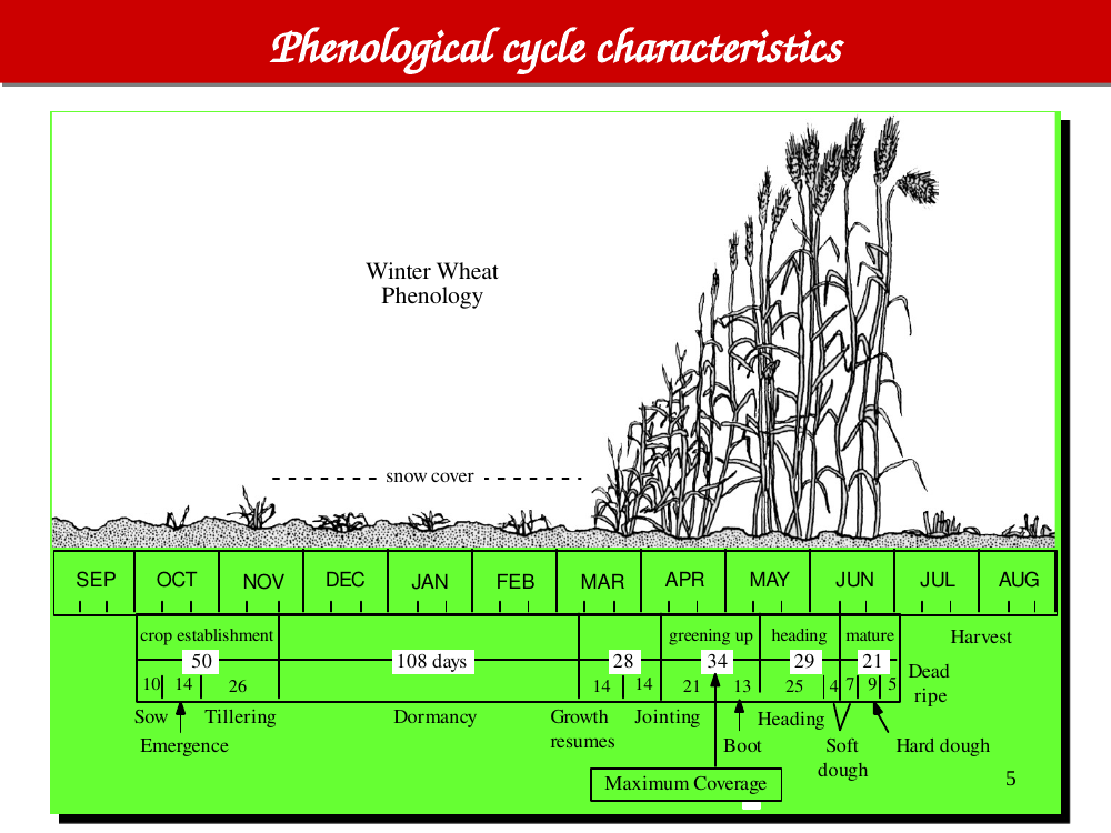
Winter wheat phenology — annual cycle

In-image text (for later study-guide use)

Title: Phenological cycle characteristics.

Subject: Winter Wheat Phenology.

Timeline (SEP → AUG):

Crop establishment (SEP–NOV): Sow / Emergence → Tillering. Days: 10, 14, 26 = ~50 days.
Dormancy (DEC–FEB): ~108 days, with snow cover.
Growth resumes (MAR): Jointing → Boot. Days: 14, 14 = 28.
Heading / greening up (APR–MAY): 21 + 13 = 34 days.
Mature (JUN): Soft dough → Hard dough → Dead ripe. 25 + 4 + 7 + 9 = ~29 days; then Harvest (+21, +5 = ~21).

Max coverage is labeled around heading / mature (APR–JUN).

Likely answer edit

Winter wheat phenology (SEP → AUG). Sow/emergence in fall → tillering → dormancy through winter (~108 days, often under snow) → growth resumes/jointing → boot → heading → dough stages → harvest in early summer.

Max vegetation signal: heading through mature (APR–JUN) — that’s when NDVI peaks.
Best imaging windows: greening-up (to separate wheat from other species) and peak cover (for biomass).

slide 6 (picture)

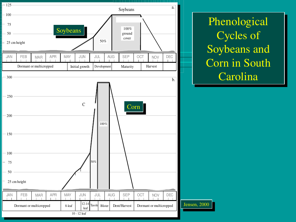
Phenological cycles — Soybeans & Corn (South Carolina)

Soybeans and corn phenological cycles, South Carolina

In-image text (for later study-guide use)

(a) Soybeans — height axis 25–125 cm; JAN–DEC timeline.
Stages: Dormant or multicropped → Initial growth → Development → Maturity → Harvest.
Ground cover rises to 50% then 100% during development/maturity.

(b) Corn — height axis 25–300 cm; JAN–DEC timeline.
Stages: Dormant or multicropped → 8-leaf → 10–12 leaf → 12–14 Tassle → Blister → Dent/Harvest → Dormant or multicropped.
Peaks at ~100% ground cover during tassle/blister.

Source: Jensen, 2000.

Likely answer edit

Soybeans & corn in South Carolina. Both are summer crops.

Soybeans — initial growth (May–June) → development → full cover at maturity (Aug–Sep) → harvest.
Corn — 8-leaf → 10–12 leaf → 12–14 leaf tassling → blister → dent/harvest by late summer.
Implication: a single June image separates winter wheat (harvested/dormant) from soybeans and corn (actively greening).

slide 7 (picture)

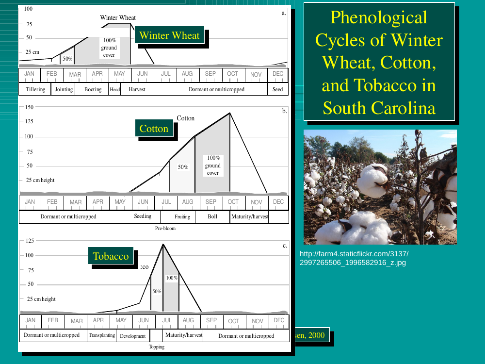
Phenological cycles — Winter Wheat, Cotton & Tobacco (South Carolina)

Winter wheat, cotton, and tobacco phenological cycles, South Carolina

In-image text (for later study-guide use)

(a) Winter Wheat — Tillering → Jointing → Booting → Head → Harvest → Dormant or multicropped → Seed.

(b) Cotton — Dormant or multicropped → Seeding → Pre-bloom → Fruiting → Boll → Maturity/harvest.

(c) Tobacco — Dormant or multicropped → Transplanting → Development → Topping → Maturity/harvest → Dormant or multicropped.

Source: Jensen, 2000.

Likely answer edit

Winter wheat, cotton, tobacco in SC — three different phenological calendars, all resolvable with a multi-date NDVI series:

Winter wheat — tiller → joint → boot → head → harvest (spring/early summer).
Cotton — seeded late spring → pre-bloom → fruiting → boll → maturity/harvest (fall).
Tobacco — transplanted spring → development → topping → harvest (summer).
Source: Jensen, 2000.

slide 8

What are vegetation indices?

A Vegetation Index (VI) is a synthetic image layer created by mathematically combining the existing bands of a multispectral image.

The new layer often surfaces information that no single band carries on its own. For example, VIs have been shown to quantify or predict:

vegetation biomass
productivity
leaf area
vegetative ground cover

Likely answer edit

A vegetation index (VI) is a synthetic band created by mathematically combining two or more bands of a multispectral image — typically NIR and red. VIs emphasize the spectral contrast between healthy vegetation (high NIR, low red) and everything else.

Used to predict: biomass, LAI, % green cover, chlorophyll content, productivity.
Key idea on the exam: a VI is derived, not measured directly.

slide 9

Normalized Difference Vegetation Index (NDVI)

NDVI is a simple numerical indicator that can be used to analyze remote-sensing measurements and assess whether the target being observed contains live green vegetation.

Likely answer edit

NDVI (Normalized Difference Vegetation Index) is the most widely used VI. It is a simple numerical indicator that assesses whether the observed target contains live green vegetation.

Developed by Rouse et al. (1974) for AVHRR imagery of the US Great Plains.
The “normalized difference” form keeps values bounded and reduces some illumination effects.

slide 10 (formula)

NDVI — value ranges

$$ \text{NDVI} = \frac{\text{NIR} - \text{Red}}{\text{NIR} + \text{Red}} $$

≤ 0.1 — barren areas of rock, sand, or snow.
0.2 – 0.3 — shrubland and grassland.
0.6 – 0.8 — temperate and tropical rainforests.

Likely answer edit

NDVI = (NIR − Red) / (NIR + Red) — ranges from −1 to +1.

NDVI	Likely surface
≤ 0.1	Barren rock, sand, snow
0.2 – 0.3	Shrubland, grassland
0.6 – 0.8	Temperate / tropical rainforest

Water is typically negative (red reflectance > NIR).
Cutoff thresholds vary by region — treat the numbers as ranges, not absolutes.

slide 11 (picture)

Vegetation reflectance curve

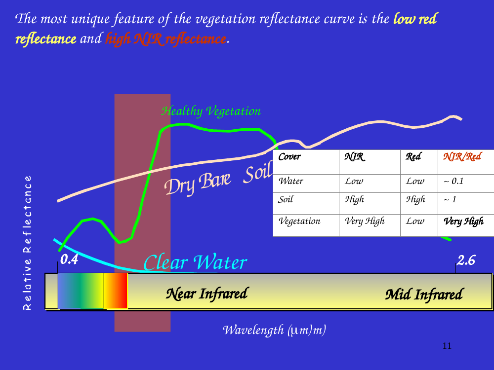
The most unique feature of the vegetation reflectance curve is the low red reflectance and high NIR reflectance.

In-image text (for later study-guide use)

Axes: Relative Reflectance (y) vs Wavelength in μm (x), range 0.4 → 2.6.

Curves shown: Healthy Vegetation (green), Dry Bare Soil (tan), Clear Water (cyan). Color spectrum bar labeled Near Infrared and Mid Infrared.

Embedded table (Cover / NIR / Red / NIR÷Red):

Water — Low / Low / ~0.1
Soil — High / High / ~1
Vegetation — Very High / Low / Very High

Likely answer edit

Vegetation reflectance curve — the defining feature of healthy vegetation is low red reflectance (chlorophyll absorbs red for photosynthesis) and high NIR reflectance (scattered by the spongy mesophyll leaf structure).

Cover	NIR	Red	NIR/Red
Water	Low	Low	~0.1
Dry bare soil	High	High	~1
Healthy vegetation	Very high	Low	Very high

That ratio contrast is why VIs like SR and NDVI work.

slide 12

Vegetation indices (VIs)

There are several VIs, and most are functionally equivalent. Nearly all combine the red and near-infrared bands:

Simple Ratio (SR)
Normalized Difference Vegetation Index (NDVI)
Enhanced Vegetation Index (EVI)

Likely answer edit

Most vegetation indices combine red and NIR bands. Three to know:

SR — Simple Ratio, NIR / Red. First true VI.
NDVI — Normalized Difference Vegetation Index, bounded −1 to 1.
EVI — Enhanced Vegetation Index, corrects for atmosphere and soil; better in dense canopies.

slide 13 (formula)

Simple Ratio (SR)

Cohen (1991) suggests that the first true vegetation index was the Simple Ratio.
Image ratioing highlights subtle variations in the spectral responses of various surface covers.
Landsat: Band 4 / Band 3.

$$ \text{SR} = \frac{\text{NIR}}{\text{Red}} $$

Likely answer edit

Simple Ratio (SR) = NIR / Red. First “true” vegetation index (Cohen 1991, building on Jordan 1969). Image ratioing highlights the spectral contrast between vegetation and non-vegetation.

On Landsat TM/ETM+, SR = Band 4 / Band 3 (NIR ÷ Red).
Weakness: unbounded; values can become very large over dense canopies, making comparisons across scenes tricky. NDVI fixes this.

slide 14 (formula)

NDVI — Rouse et al. (1974)

NDVI values are real numbers in the range −1 to 1:

Well-vegetated areas have higher values (NIR ≫ red reflectance).
Water (and sometimes shadow) has negative values (red > NIR reflectance).
Rock, dry soil, senesced vegetation hover near zero (red ≈ NIR reflectance).

$$ \text{NDVI} = \frac{\text{NIR} - \text{Red}}{\text{NIR} + \text{Red}} $$

Likely answer edit

NDVI = (NIR − Red) / (NIR + Red) — developed by Rouse et al. (1974), ranges −1 to 1.

Well-vegetated pixels have high values (NIR ≫ Red).
Water / shadow have negative values (Red > NIR).
Rock, dry soil, senesced veg. are near zero (Red ≈ NIR).
On Landsat TM/ETM+: NDVI = (B4 − B3) / (B4 + B3). On Landsat 8/9 OLI: (B5 − B4) / (B5 + B4).

slide 15 (picture)

Example NDVI image

In-image text (for later study-guide use)

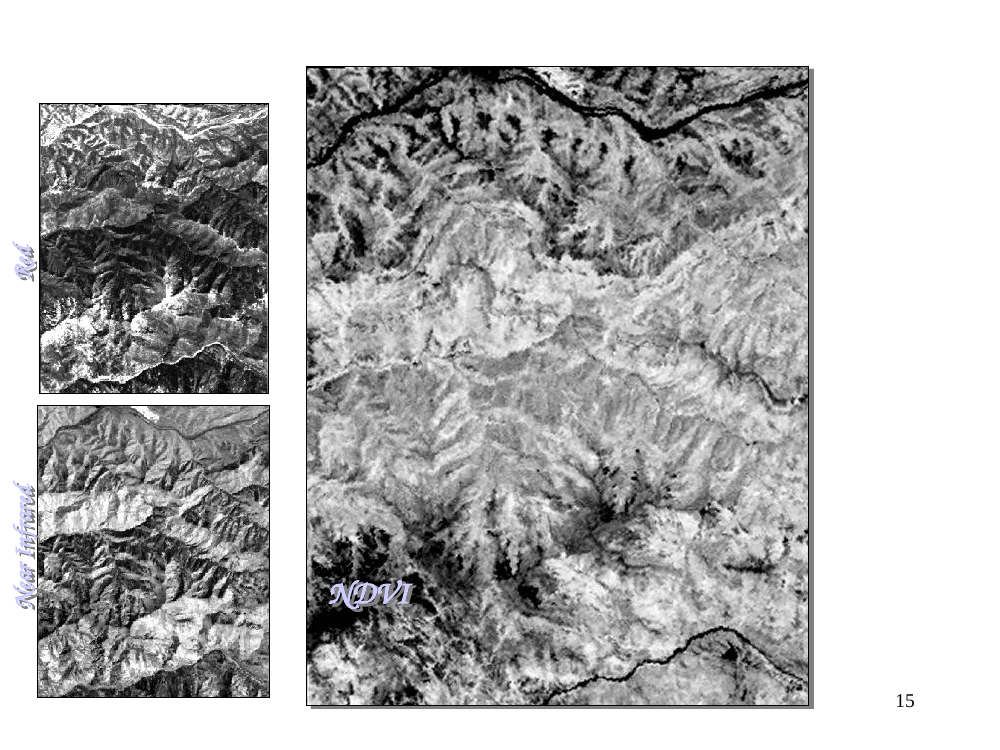
Three panels: Red band (top-left), Near Infrared band (bottom-left), and the resulting NDVI (right). Scene is mountainous terrain rendered in grayscale.

Likely answer edit

Example three-band panel — the Red band alone, the NIR band alone, and the computed NDVI. Vegetated slopes appear dark in Red, bright in NIR, and bright in NDVI.

This visualizes why the index “works”: the combination of the two raw bands makes vegetation pop out in a way neither band does on its own.

slide 16 (picture)

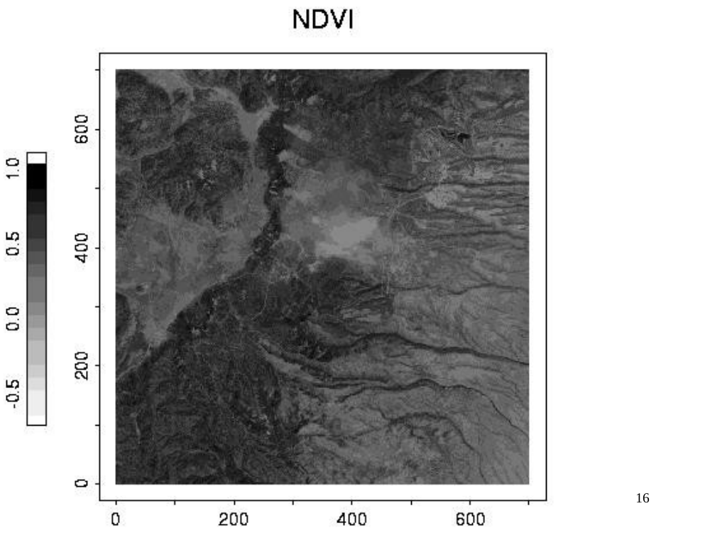
NDVI image

In-image text (for later study-guide use)

Title NDVI. Grayscale raster, axes 0–600 (x) and 0–800 (y) pixels. Left-side color bar from −0.5 to 1.0.

Likely answer edit

NDVI grayscale image. Higher NDVI = brighter pixel. Spatial patterns trace land cover boundaries (forest vs. cropland vs. bare ground) better than any single spectral band.

Scale bar from roughly −0.5 to 1.0 — anything negative is water or shadow.

slide 17 (picture)

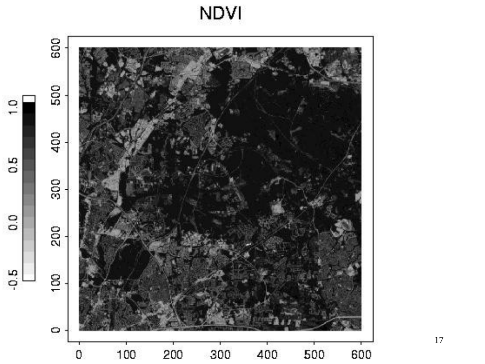
NDVI image (second scene)

In-image text (for later study-guide use)

Title NDVI. Grayscale raster, axes 0–600 on both x and y. Left-side color bar from −0.5 to 1.0. Appears to cover a different (flatter, possibly urbanized) scene than slide 16.

Likely answer edit

A second NDVI example (different scene). Shows how an NDVI image quickly discriminates vegetated vs. non-vegetated / built-up areas even at moderate resolution.

slide 18 (picture)

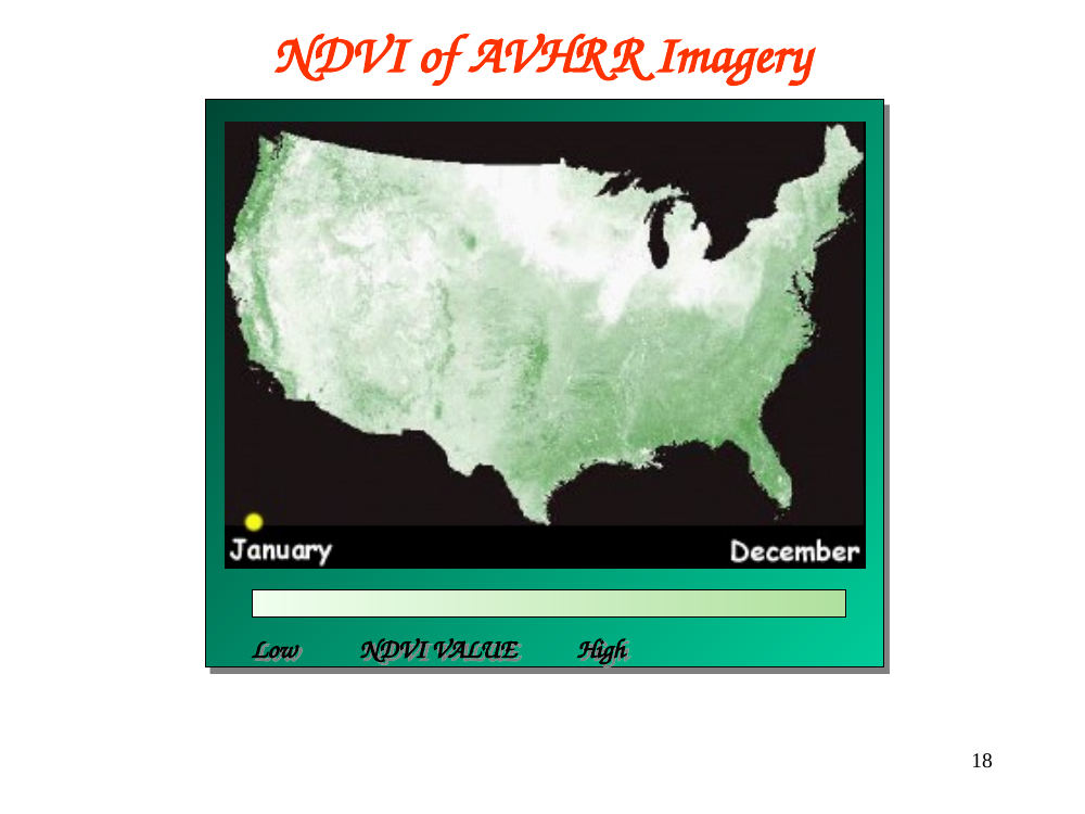
NDVI of AVHRR imagery — seasonal progression

In-image text (for later study-guide use)

Title NDVI of AVHRR Imagery. US map colored by NDVI, annotated Progression through the season…. Timeline runs from January (left) to December (right). Color bar: Low NDVI VALUE → High.

Likely answer edit

NDVI of AVHRR imagery — seasonal progression of the continental US (Jan → Dec).

Coast and southern states stay green year-round; the Midwest pulses with the growing season.
Use case: monitoring drought, crop health, and broad-scale phenological shifts at continental scale with ~1 km AVHRR data.

slide 19 (formula)

Enhanced Vegetation Index (EVI)

$$ \text{EVI} = \frac{R_{\text{NIR}} - R_{\text{Red}}}{R_{\text{NIR}} + C_1 R_{\text{Red}} - C_2 R_{\text{Blue}} + L}\,(1 + L) $$

$C_1$, $C_2$ — coefficients adjusting for atmospheric (aerosol) effects.
$L$ — soil adjustment factor.
Empirically determined as $C_1 = 6.0$, $C_2 = 7.5$, $L = 1.0$.
EVI has improved sensitivity to high-biomass regions (where NDVI saturates).

Source: Huete and Justice, 1999, MODIS Vegetation Index Algorithm Theoretical Basis Document.

Likely answer edit

EVI corrects NDVI’s main weaknesses — atmospheric aerosol scattering (via the blue band) and soil-background brightness (via the L term).

EVI = [(NIR − Red) / (NIR + C1·Red − C2·Blue + L)] × (1 + L)

With C1 = 6.0, C2 = 7.5, L = 1.0 (MODIS standard).

Improved sensitivity in high-biomass regions where NDVI saturates.
Requires a blue band — not every sensor has one, but MODIS, Landsat 8/9, and Sentinel-2 do.

slide 20

Beyond standard VIs — linear transformations

In addition to the standard VIs, several transformation equations each create a new set of derived images:

PCA — Principal Component Analysis.
K-T — Kauth-Thomas "Tasseled Cap" transform.

Likely answer edit

Beyond ratios, two linear transformations to know:

PCA (Principal Component Analysis) — decorrelates bands into components ordered by variance. PC1 usually captures brightness; later PCs isolate features (e.g., vegetation).
K-T (Kauth-Thomas) “Tasseled Cap” — a fixed linear transform tuned for Landsat that produces interpretable axes: Brightness, Greenness, Wetness (and sometimes a 4th).