Multispectral scanning geometries — the two big families.
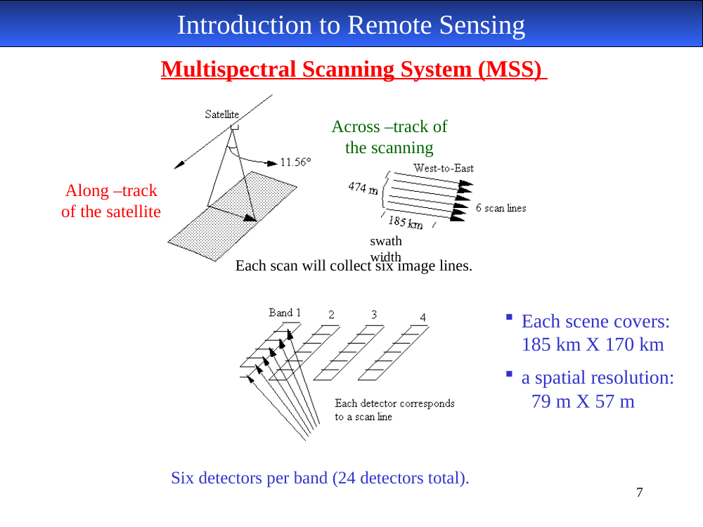
Across-track (“whiskbroom”) — discrete detectors + a scanning mirror sweep perpendicular
to flight. Examples: Landsat MSS, TM, ETM+.
Along-track (“pushbroom”) — a linear array of detectors builds the image as the
platform moves forward. Examples: SPOT HRV/HRVIR, IRS LISS, IKONOS, QuickBird, Landsat 8/9 OLI.
Sensors span roughly 0.4–14 µm (visible through thermal-IR).
slide 4 (picture)
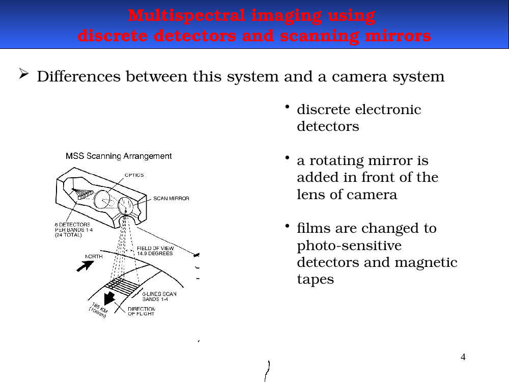
Multispectral scanner vs. a camera
In-image text (for later study-guide use)
Differences called out in the diagram:
Uses discrete electronic detectors.
A rotating mirror is added in front of the camera lens.
Film is replaced by photo-sensitive detectors recording to magnetic tape.
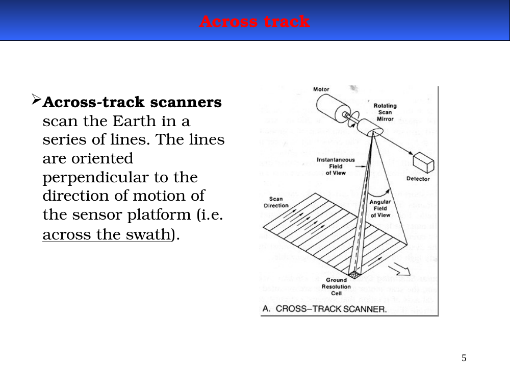
Across-track scanner motion. Scans the Earth in a series of lines perpendicular to the
flight path — i.e., across the swath. The platform’s forward motion moves the next scan
line along-track. Combined, this builds a 2D image.
slide 6 (picture)
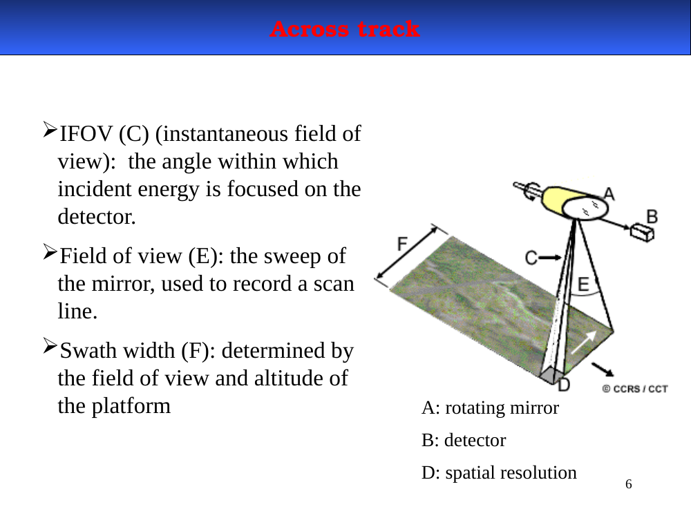
Across-track terminology — IFOV, FOV, swath
In-image text (for later study-guide use)
A — rotating mirror.
B — detector.
C (IFOV) — instantaneous field of view: the angle within which incident energy is focused on one detector.
D — spatial resolution (ground pixel size from IFOV × altitude).
E (FOV) — sweep angle of the full mirror swing, one scan line.
Across-track scanner terminology (memorize all four):
IFOV (Instantaneous Field of View) — the angle within which incident energy is focused
on the detector at one moment. Combined with altitude, it determines spatial resolution
(the ground pixel size).
Field of view (FOV) — the full sweep angle of the mirror, defining a complete scan line.
Swath width — on-ground width of one scan line; set by FOV × altitude.
Diagram labels: A = rotating mirror, B = detector, C = IFOV, D = spatial
resolution, E = FOV, F = swath width.
Along-track scanner motion. A linear detector array perpendicular to flight records a
whole swath line in one look. The aircraft’s/satellite’s forward motion advances to the next line.
Because there’s no moving mirror, along-track is mechanically simpler and more reliable.
slide 9 (picture)
Pushbroom geometry
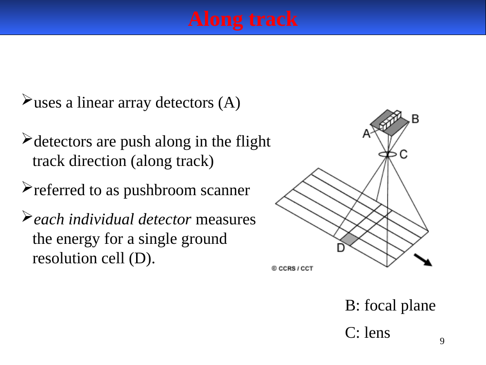
Uses a linear array of detectors (A).
Detectors are "pushed along" in the flight direction — hence pushbroom.
Each individual detector measures energy for a single ground resolution cell (D).
In-image text (for later study-guide use)
Labels: A linear array detectors, B focal plane, C lens, D ground resolution cell.
Linear detector array (A) sits perpendicular to the flight direction.
Detectors are “pushed along” as the platform moves — hence “pushbroom.”
Each detector samples one ground resolution cell (D) per integration period.
Labels: B = focal plane, C = lens.
slide 10 (picture)
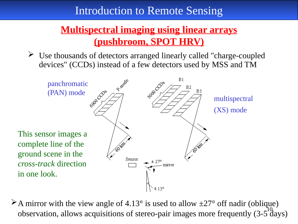
SPOT HRV pushbroom — PAN and XS modes
Uses thousands of CCDs arranged linearly — vastly more detectors than MSS/TM. Images a complete cross-track line in one look. A steerable mirror (view angle 4.13°) enables ±27° off-nadir viewing → stereo and 3–5 day revisit.
In-image text (for later study-guide use)
Two stacked linear arrays depicted: a panchromatic (PAN) mode array and a multispectral (XS) mode array (one sub-array per band). A single steerable mirror feeds both.
Pushbroom (linear) vs. whiskbroom (scanning) — why pushbroom is superior.
No moving mirror → more reliable, longer mission life.
Longer dwell time per pixel → higher signal-to-noise, stronger signal.
CCDs are smaller, lighter, lower-power than the optics a scanning mirror needs.
Disadvantage of pushbroom: calibrating thousands of detectors to produce a uniform
radiometric response is difficult (each CCD has slightly different gain/offset) — a given
scanner with one detector never has this problem.
slide 12
Satellite orbits
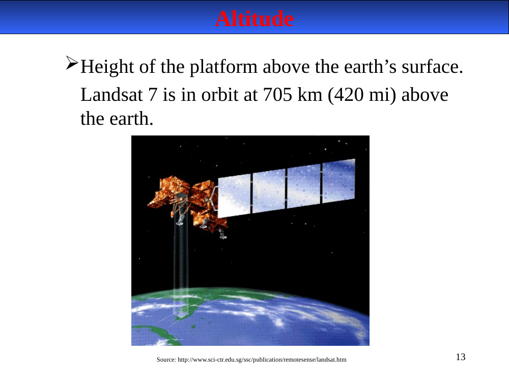
An orbit is the path followed by a satellite. Four descriptors:
Landsat 1–3 (earlier orbit): 919 km — lowered to 705 km starting with Landsat 4 to
improve spatial resolution.
slide 14 (picture)
Period — orbits per day
Time to complete one orbit. Landsat 7: 99 min → 14.5 orbits per day.
In-image text (for later study-guide use)
Latitude vs. longitude grid showing 14.5 successive orbit tracks in one day. Latitudes marked 0° through 75° (N). Orbit numbers 1–15 visible across the chart. Source: Jensen, 2000.
Sun-synchronous orbit. A special near-polar orbit tuned so that the orbital plane
precesses at the same angular rate Earth revolves around the Sun.
Consequence: the satellite crosses the equator at the same local solar time every
day — typically between 9:30 and 10:00 AM for Landsat/SPOT, so illumination
conditions are consistent across acquisitions.
slide 19
Geostationary orbits
Altitude ~36 000 km above the equator.
Orbital period matches Earth's rotation → satellite appears stationary over one longitude.
Landsat 8 and 9 fly offset by 8 days (not 12 h as some older slides state), giving
the combined constellation an 8-day effective revisit.
Both carry OLI + TIRS (OLI-2 + TIRS-2 on Landsat 9).
slide 22
Landsat continuity timeline
Original slide graphic (NASA timeline image) was lost during PDF conversion. Conceptual summary follows.
Landsat has provided continuous Earth imagery since 1972 — the longest-running civilian Earth-observation record. The series has overlapped missions deliberately so there is never a coverage gap.
Landsat continuity timeline. The original slide’s graphic was lost in PDF conversion.
In short: the Landsat program has provided continuous Earth imagery since 1972, with
at least one operational satellite at almost every moment.
Current operational pair: Landsat 8 (2013) + Landsat 9 (2021).
Landsat Next is planned for launch ~2030 with 26 bands at higher temporal cadence.
Landsat 7 ETM+ band table. The original slide’s embedded table did not survive PDF
conversion — the full table is on slide 27 (above). Key point to remember: Landsat 7
bands are at slightly different wavelengths than Landsat 5 TM (small recalibration).
slide 30
Landsat band properties — what each is good for
1 — Blue, 0.45 – 0.52 µm. Coastal water mapping, soil/vegetation discrimination, forest type, cultural features.
2 — Green, 0.52 – 0.60 µm. Vegetation ID and vigor; cultural features.
3 — Red, 0.63 – 0.69 µm. Plant species discrimination; soil / geologic boundaries; cultural features.
Landsat 9 — OLI-2 + TIRS-2. Launched Sept 27, 2021. The original slide’s table
didn’t survive conversion; here is the full band list (same geometry as Landsat 8 OLI):
Band
Name
Wavelength
Resolution
1
Coastal / Aerosol
0.43 – 0.45 µm
30 m
2
Blue
0.45 – 0.51 µm
30 m
3
Green
0.53 – 0.59 µm
30 m
4
Red
0.64 – 0.67 µm
30 m
5
NIR
0.85 – 0.88 µm
30 m
6
SWIR-1
1.57 – 1.65 µm
30 m
7
SWIR-2
2.11 – 2.29 µm
30 m
8
Panchromatic
0.50 – 0.68 µm
15 m
9
Cirrus
1.36 – 1.38 µm
30 m
10
Thermal-1 (TIRS-2)
10.6 – 11.19 µm
100 m (resampled to 30)
11
Thermal-2 (TIRS-2)
11.5 – 12.51 µm
100 m (resampled to 30)
14-bit quantization, higher SNR than L7/L8.
Note the OLI band-numbering shift vs. TM: Blue is now Band 2 (not 1), because
Band 1 was added for coastal/aerosol.
slide 33 (picture)
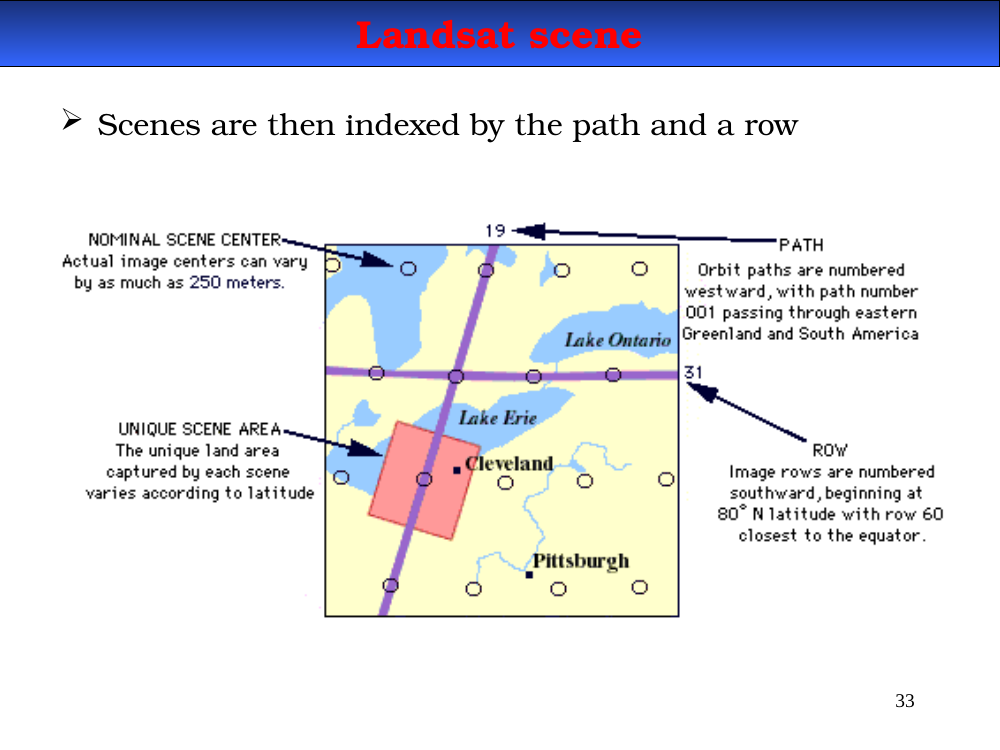
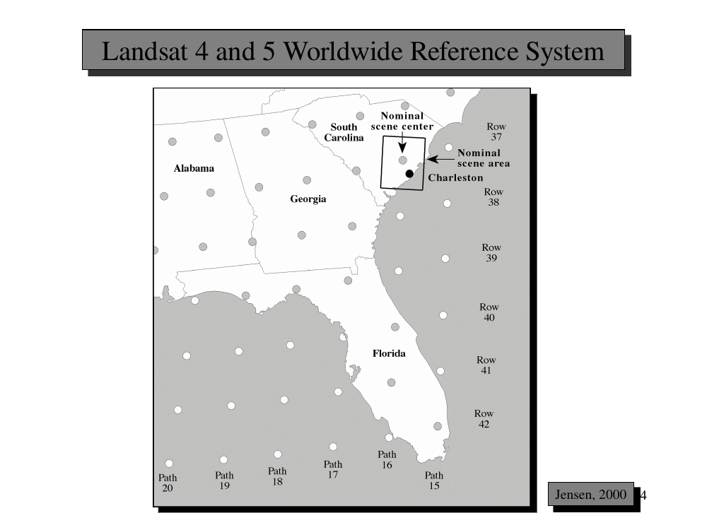
Landsat scene — indexed by Path and Row
In-image text (for later study-guide use)
PATH — orbit paths are numbered westward; Path 001 passes through eastern Greenland and South America.
ROW — image rows are numbered southward, beginning at 80°N latitude; Row 60 is closest to the equator.
Nominal scene center — actual image centers can vary by as much as 250 m.
Unique scene area — the unique land covered by each scene varies with latitude.
Example on the diagram: Path 19, Row 31 over Lake Erie / Cleveland / Pittsburgh.
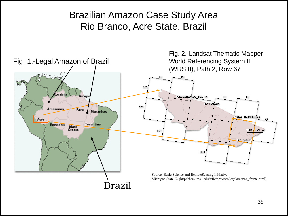
Site: Rio Branco, Acre State, western Brazilian Amazon.
Path / Row: WRS-2 Path 2, Row 67.
Shown in two context maps: (1) the “Legal Amazon” region of Brazil; (2) the WRS-2 grid
cell marking the specific Landsat scene over Rio Branco.
Why Rio Branco: classic demonstration site for Landsat deforestation time series — the
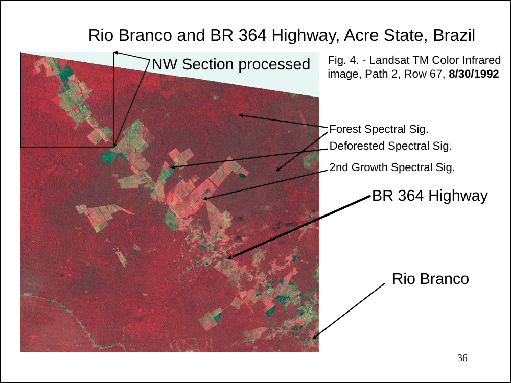
BR 364 highway triggered rapid forest clearing in the 1970s–90s.
slide 36 (picture)
Rio Branco CIR image — deforestation signatures
In-image text (for later study-guide use)
Title: Rio Branco and BR 364 Highway, Acre State, Brazil.