Unsupervised Classification — ISODATA
Classification schemes (Anderson LULC), the ISODATA algorithm, and its three parameters.
Image classification — the idea
A process of assigning each pixel in an image to one of a number of classes. The result is a thematic map.
Image classification — the big idea. A process of assigning every pixel in an image to one of a pre-defined set of classes. The output is a thematic map (e.g., forest / crop / water / urban).
- Two broad families: unsupervised (this deck) and supervised (next deck).
Unclassified vs. classified
In-image text (for later study-guide use)
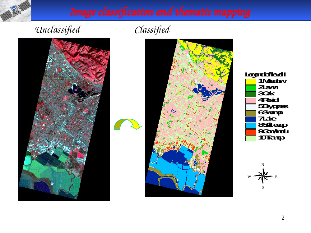
Left: raw multispectral image. Right: classified thematic map. Legend, Level 1: 1 Meadow, 2 Lawn, 3 Oak, 4 Residential, 5 Dry grass, 6 Swamp, 7 Lake, 8 Salt evap, 9 Comm/Industrial, 10 Transportation. Compass rose N / W / E / S on the right-hand side.
Unclassified vs. classified. Left: the raw multispectral image with 11 classes in the legend (Meadow, Lawn, Oak, Residential, Dry grass, Swamp, Lake, Salt evap, Comm/Indu, Transportation…). Right: the same scene after classification — each pixel assigned to one of those classes, shown as a flat color.
- A good thematic map has tight spectral separability between classes and an accuracy assessment to back it up (see slide 3).
Classification process — three steps
- A classification scheme
- Classification methods
- Accuracy assessment
Three steps of any classification project.
- Classification scheme — define the classes (and hierarchy) up front.
- Classification methods — pick the algorithm (ISODATA, K-means, Max Likelihood, etc.).
- Accuracy assessment — confusion matrix, user’s / producer’s accuracy, kappa.
Classification process (recap)
- A classification scheme
- Classification methods
- Accuracy assessment
(Repeat of slide 3 in the original deck.) Same three-step outline — the instructor uses it as a navigation anchor for the rest of the lecture.
Classification schemes
- Classes are always a simplification and generalization of reality.
- Scheme depends on the information-extraction objective.
- Can be broad / abstract or specific / concrete.
- Hierarchical systems are standard — coarse → fine.
- Canonical example: Anderson (1976) LULC system — Level I 9 classes, Level II 37 subclasses.
Choosing a classification scheme.
- Classes are always a simplification / generalization of the real world.
- Scheme choice depends on the information-extraction objective (are you counting tree crowns, or mapping land cover?).
- You can pick broad/abstract or specific/concrete classes.
- Hierarchical schemes are standard — coarse top level → refined sub-classes.
- Canonical example: Anderson (1976) land-use / land-cover system for RS data. Level I = 9 classes; Level II = 37 subclasses.
Anderson LULC — Level I: 1–4
| Level I | Level II |
|---|---|
| 1 Urban / Built-up | 11 Residential, 12 Commercial & Services, 13 Industrial, 14 Transportation / Communications / Utilities, 15 Industrial + Commercial Complexes, 16 Mixed Urban, 17 Other Urban |
| 2 Agricultural | 21 Cropland & Pasture, 22 Orchards/Groves/Vineyards/Nurseries/Horticulture, 23 Confined Feeding, 24 Other Agricultural |
| 3 Rangeland | 31 Herbaceous, 32 Shrub & Brush, 33 Mixed |
| 4 Forest | 41 Deciduous, 42 Evergreen, 43 Mixed |
Anderson LULC — Level I (1–4) classes.
| Level I | Level II |
|---|---|
| 1 Urban or Built-up | 11 Residential, 12 Commercial, 13 Industrial, 14 Transportation/Communications/Utilities, 15 Industrial + Commercial Complexes, 16 Mixed Urban, 17 Other Urban |
| 2 Agricultural | 21 Cropland & Pasture, 22 Orchards/Vineyards/Horticulture, 23 Confined Feeding, 24 Other Agricultural |
| 3 Rangeland | 31 Herbaceous, 32 Shrub & Brush, 33 Mixed |
| 4 Forest | 41 Deciduous, 42 Evergreen, 43 Mixed |
Anderson LULC — Level I: 5–9
| Level I | Level II |
|---|---|
| 5 Water | 51 Streams & Canals, 52 Lakes, 53 Reservoirs, 54 Bays & Estuaries |
| 6 Wetland | 61 Forested Wetland, 62 Nonforested Wetland |
| 7 Barren Land | 71 Dry Salt Flats, 72 Beaches, 73 Sandy areas not beaches, 74 Bare Exposed Rock, 75 Strip Mines / Quarries / Gravel Pits, 76 Transitional, 77 Mixed Barren |
| 8 Tundra | 81 Shrub & Brush, 82 Herbaceous, 83 Bare Ground, 84 Wet, 85 Mixed |
| 9 Perennial Snow / Ice | 91 Perennial Snowfields, 92 Glaciers |
Anderson LULC — Level I (5–9) classes.
| Level I | Level II |
|---|---|
| 5 Water | 51 Streams & Canals, 52 Lakes, 53 Reservoirs, 54 Bays & Estuaries |
| 6 Wetland | 61 Forested, 62 Nonforested |
| 7 Barren Land | 71 Dry Salt Flats, 72 Beaches, 73 Sandy areas not beaches, 74 Bare Rock, 75 Strip Mines/Quarries, 76 Transitional, 77 Mixed Barren |
| 8 Tundra | 81 Shrub & Brush, 82 Herbaceous, 83 Bare Ground, 84 Wet, 85 Mixed |
| 9 Perennial Snow / Ice | 91 Perennial Snowfields, 92 Glaciers |
Classification process (section marker)
- A classification scheme
- Classification methods
- Accuracy assessment
(Step navigation slide.) Same three-step outline — moving from “scheme” to “methods.”
Multispectral classification
- Makes use of spectral response patterns of ground objects.
- Per-pixel (point) classifiers — decide each pixel independently.
- The heart of RS for land-cover discrimination.
Multispectral (per-pixel) classification.
- Makes use of spectral response patterns — different land-cover types reflect different amounts in each band, creating separable “clusters” in feature space.
- Per-pixel / point classifiers look at one pixel at a time (no spatial context).
- This approach is the heart of remote-sensing land-cover work, despite not using neighborhood information.
Spectral reflectance curves
Different types of Earth-surface features have their own distinctive EM reflectance signatures. That's why classification works.
Spectral reflectance curves. Different surface features have distinctive EM reflectance “signatures” across wavelength. That’s why band math and classification work at all.
- Vegetation: low red, high NIR.
- Water: low everywhere, especially NIR.
- Soil: moderate across the board, peaks in SWIR.
- Snow: high in visible, drops in SWIR (how we separate snow from clouds).
Supervised vs. unsupervised classification
| Supervised | Unsupervised | |
|---|---|---|
| Typical algorithm | Maximum Likelihood | ISODATA |
| A priori knowledge | Required | Not required |
| Control | More controlled by the user | More computer-automated |
Supervised vs. unsupervised — side-by-side comparison.
| Supervised | Unsupervised | |
|---|---|---|
| Typical algorithm | Maximum Likelihood | ISODATA |
| A priori knowledge | Required (training sites) | Not required |
| Control | More user control | More computer-automated |
- Classic trade-off: unsupervised is quick and reveals natural groupings; supervised is more accurate when you have good training data.
Unsupervised classification (clustering)
- User supplies only a few parameters.
- The computer uncovers statistical patterns (similar spectral characteristics) inherent in the data.
- Spectral classes don't necessarily correspond to meaningful ground-object categories — the analyst must attach real-world labels afterward.
Unsupervised classification (clustering) — how it differs from supervised.
- User supplies only a few parameters; no training sites.
- Computer finds statistical patterns (spectral clusters) in the data automatically.
- Spectral classes ≠ meaningful categories. The output is “Cluster 7”, not “Corn.”
- Post-labeling is required — the analyst assigns real-world labels to each cluster after the algorithm runs (often via the Recode tool).
ISODATA — Iterative Self-Organizing Data Analysis Technique
- Uses minimum spectral distance to assign a cluster to every candidate pixel.
- Iterative — repeatedly reclassifies every pixel and recomputes cluster statistics.
Source: ERDAS Field Guide 2002, Fig. 6-12, p. 232.
ISODATA — Iterative Self-Organizing Data Analysis Technique.
- Assigns each candidate pixel to its closest cluster mean (minimum spectral distance).
- Iterative: repeatedly re-classifies every pixel and recomputes cluster statistics until stable.
- Derived from ERDAS Imagine’s implementation (Field Guide 2002 p. 232).
Three ISODATA parameters — N, T, M
- N — maximum number of clusters (also the maximum number of classes).
- T — convergence threshold. The % of pixels whose class values must stay unchanged between iterations for ISODATA to declare it's done.
- M — maximum number of iterations to perform.
ISODATA — three parameters the user must set.
- N — max number of clusters. Becomes the maximum possible number of classes.
- T — convergence threshold. The % of pixels whose class values must stay unchanged between iterations to declare convergence (e.g., 95%, 98%).
-
M — max iterations. Safety limit so the algorithm halts even if T is never reached.
- Rule of thumb: if ISODATA returns far fewer clusters than N, your data doesn’t support that many; if it maxes out N, bump the parameter up.
T — convergence threshold — worked example
After each iteration, the normalized percentage of pixels whose assignments are unchanged is calculated.
| Pixel | Class value, previous iteration | Class value, current iteration | Change of class value |
|---|---|---|---|
| 1 | 1 | 1 | 0 |
| 2 | 2 | 2 | 0 |
| 3 | 3 | 3 | 0 |
| 4 | 4 | 4 | 0 |
| 5 | 4 | 3 | 1 |
| 6 | 3 | 4 | 1 |
| 7 | 2 | 1 | 1 |
| 8 | 2 | 2 | 0 |
| 9 | 3 | 3 | 0 |
| 10 | 4 | 4 | 0 |
# pixels changed = 3
# pixels unchanged = 7
T (unchanged % of pixel reassignments):
= # unchanged ÷ total # of pixels
= 7 / 10 = 70%
If the user set T = 95%, ISODATA would iterate again (70% < 95%).
Worked example — computing the convergence threshold T.
The slide’s 10-pixel table shows which pixels changed class between iterations:
| Pixel | Prev class | Current class | Changed? |
|---|---|---|---|
| 1 | 1 | 1 | 0 |
| 2 | 2 | 2 | 0 |
| 3 | 3 | 3 | 0 |
| 4 | 4 | 4 | 0 |
| 5 | 4 | 3 | 1 |
| 6 | 3 | 4 | 1 |
| 7 | 2 | 1 | 1 |
| 8 | 2 | 2 | 0 |
| 9 | 3 | 3 | 0 |
| 10 | 4 | 4 | 0 |
- Changed: 3 pixels. Unchanged: 7 pixels.
- T (unchanged %) = unchanged ÷ total = 7 / 10 = 70%.
- If the operator set T = 95%, 70% is not yet high enough → ISODATA runs another iteration.
ISODATA procedure (1)
- Determine N arbitrary cluster means to start.
- Compute the spectral distance between each candidate pixel and every cluster mean.
- Assign each pixel to its closest cluster mean.
- After each iteration, recalculate each cluster mean from the actual pixel membership — means shift in feature space.
- Use the new means for the next iteration.
ISODATA procedure, part 1 — the first pass.
- Pick N arbitrary cluster means to start.
- Compute the spectral distance between each pixel and every cluster mean.
- Assign each pixel to its closest mean.
- After the pass, recompute each cluster’s mean using the actual pixels that ended up in it — the means shift in feature space.
- Use the new means for the next iteration.
ISODATA procedure (2)
- The process repeats — each candidate pixel compared to the new cluster means and reassigned to the closest.
- Terminates when either the convergence threshold T is reached OR the maximum number of iterations M is reached.
ISODATA procedure, part 2 — iteration and termination.
- Each new iteration: compare every pixel to the updated means, reassign to the closest cluster.
- Stop condition — whichever comes first:
- Convergence threshold T is reached (few pixels moving classes).
- Max iterations M is reached.
ISODATA clustering procedure — three snapshots
In-image text (for later study-guide use)
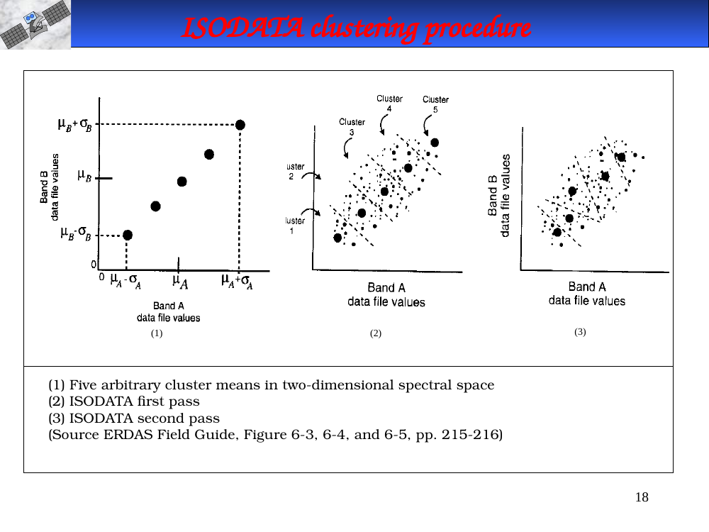
- (1) Five arbitrary cluster means in two-dimensional spectral space.
- (2) ISODATA first pass.
- (3) ISODATA second pass.
Source: ERDAS Field Guide, Figures 6-3, 6-4, 6-5, pp. 215–216.
ISODATA visualization — three snapshots.
- (1) Five arbitrary initial cluster means plotted in 2-D spectral space.
- (2) After the first pass — cluster means have shifted toward the actual pixel densities.
- (3) Second pass — means have stabilized closer to true cluster centers.
Source: ERDAS Field Guide, Figures 6-3/6-4/6-5, pp. 215–216.
Deck: Ma_2024_RS8-UnsupervisedClassification.ppt — 18 slides.
Download original
·
Edit our reproduction