Sensors — SPOT & IKONOS
Scanning geometries, the SPOT 1–7 family, and the first sub-meter commercial satellite.
SPOT image — what can you distinguish?
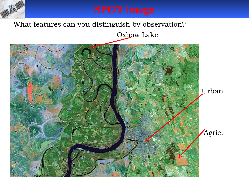
In-image text (for later study-guide use)
Three labels annotated on the scene:
- Oxbow Lake — a sinuous cutoff river meander.
- Urban — developed area, geometric bright patches.
- Agric. — agricultural fields.
SPOT scene interpretation practice. The example shows three land-cover classes you should be able to pick out from a SPOT multispectral image:
- Oxbow lake — dark sinuous water feature (river meander cutoff).
- Urban — bright, geometric patterns.
- Agriculture — regular rectangular fields, often in false color due to NIR vegetation response.
Scene footprint — SPOT HRV vs. Landsat TM/MSS
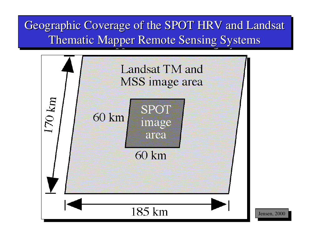
In-image text (for later study-guide use)
Diagram compares two scene sizes:
- SPOT HRV image area — 60 km × 60 km.
- Landsat TM / MSS image area — 185 km × 170 km (Landsat TM swath 185 km).
Source: Jensen, 2000.
Scene-size comparison. The illustration contrasts the footprint of a single image:
- SPOT HRV: 60 km × 60 km
-
Landsat TM / MSS: 185 km × 170 km
- Trade-off: SPOT’s smaller scene gives higher resolution; Landsat’s larger scene covers more ground per pass, so fewer scenes are needed to mosaic a region.
IKONOS Traverse Bay overview — data volumes
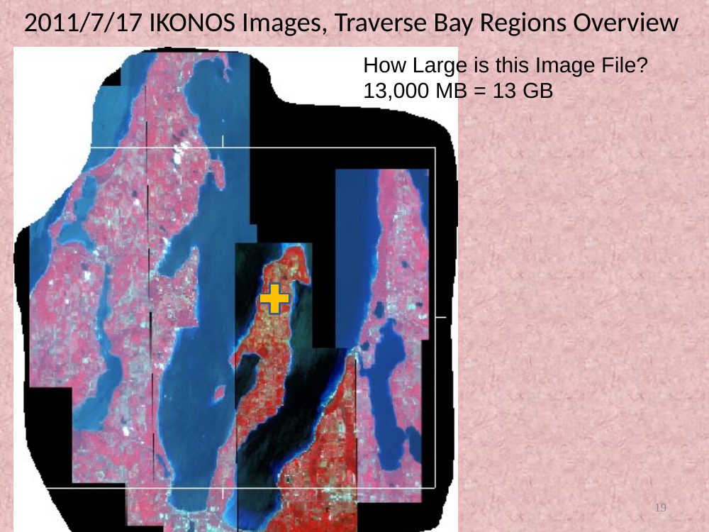
In-image text (for later study-guide use)
Title: 2011/7/17 IKONOS Images, Traverse Bay Regions Overview.
Annotation: How Large is this Image File? 13 000 MB = 13 GB.
Data-volume takeaway. The IKONOS image of Traverse Bay is 13 000 MB (13 GB) for a single high-resolution mosaic. High spatial + high radiometric (11-bit) + multi-band = huge files. Plan storage and processing for any high-resolution project.
Pan-sharpened example — Old Mission Point orchards
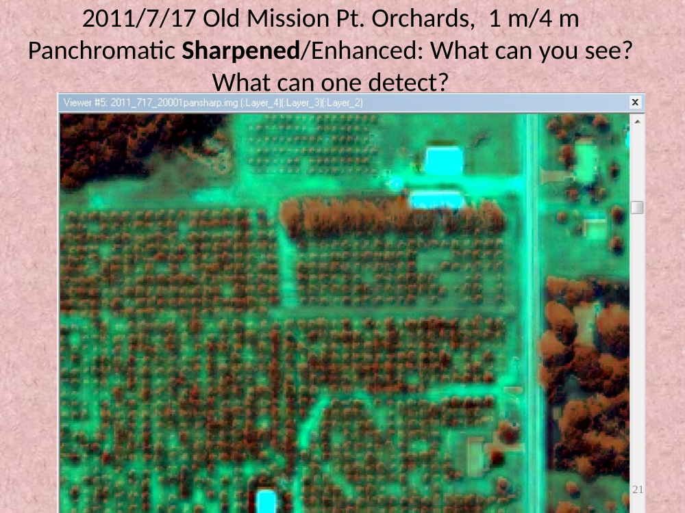
In-image text (for later study-guide use)
Title: 2011/7/17 Old Mission Pt. Orchards, 1 m/4 m Panchromatic Sharpened/Enhanced: What can you see? What can one detect?
Pan-sharpening fuses the 1 m panchromatic band with the 4 m multispectral bands to yield an effective 1 m color image.
Pan-sharpened example — Old Mission Point Orchards (2011). The 1 m panchromatic is fused with the 4 m multispectral to yield a 1 m color image. Typical things you can now detect:
- Individual trees and tree rows in the orchards.
- Buildings, driveways, vehicles, fences.
- Crop vigor differences via the multispectral component.
Pan-sharpening is a standard IKONOS workflow — trades a little spectral fidelity for major spatial detail.
Deck: 2023RemoteSensingSensors-Spot-IkonosRevV2.ppt — 19 slides.
Download original
·
Edit our reproduction