Supervised Classification
Training samples → signatures → decision rules. All formulas rendered.
Supervised classification — setup
Supervised classification requires a priori knowledge about the image data:
- Which types of land-use exist in the study area.
- Geographical locations of reliable samples for each land-use type.
Supervised classification — the setup. Requires a priori knowledge about the scene:
- Which land-use types exist in the study area.
- The geographic location of reliable samples (training sites) for each class.
Without good training data, supervised classification fails. Garbage in, garbage out.
Procedure — three steps
- Selection of training samples
- Generation and evaluation of statistical signatures
- Class assignment using a decision rule
Three-step supervised procedure.
- Select training samples — homogeneous AOIs for each class.
- Generate and evaluate statistical signatures — mean, std, covariance per band, per class.
- Class assignment using a decision rule — Parallelepiped, Min Distance, Max Likelihood, or Mahalanobis.
Training samples
- Samples of homogeneous areas with known class types.
- Selection methods: fieldwork, aerial photography, maps, personal experience.
- Spectral characteristics of training samples are used to generate signatures.
Training samples — the foundation.
- Must be homogeneous areas of known class (land-use) type.
- Ways to pick them:
- Fieldwork (ground truthing with GPS).
- Aerial photography at higher resolution than the sensor being classified.
- Existing maps / GIS layers.
- Personal experience / local knowledge.
- Their spectral characteristics are then used to generate the class signatures.
Parametric signatures
- Multivariate statistical parameters per class: min, max, mean, standard deviation, variance, covariance.
- Each signature corresponds to a class, and is used with a decision rule to assign pixels.
- Signatures can be evaluated, deleted, renamed, or merged.
Parametric signatures.
- Each class gets a multivariate statistical summary:
- Min / max
- Mean
- Standard deviation
- Variance
- Covariance (across bands)
- Each signature is paired with a decision rule to classify pixels.
- Signatures can be evaluated, deleted, renamed, or merged before running the classifier.
Mean, standard deviation, variance — worked example
Water signature with three pixels in two bands: (24, 3), (26, 5), (28, 10).
Standard deviation (k pixels):
- where i is a particular pixel and k is the number of pixels.
- Band 1:
S_Q₁ = 2 - Band 2:
S_Q₂ = 3.6
Variance is the squared standard deviation:
- Variance of Band 1 = 4
- Variance of Band 2 = 12.96
Mean, standard deviation, variance — worked example (water class, 3 pixels, 2 bands).
Pixels: (24, 3), (26, 5), (28, 10). Band 1 values: 24, 26, 28. Band 2 values: 3, 5, 10.
\[\bar{Q}_1 = \frac{24 + 26 + 28}{3} = 26 \qquad \bar{Q}_2 = \frac{3 + 5 + 10}{3} = 6\]Standard deviation formula (k pixels):
\[S_Q \;=\; \sqrt{\frac{\sum_{i=1}^{k} (Q_i - \bar{Q})^2}{k-1}}\]- Band 1:
S_Q₁ = 2 - Band 2:
S_Q₂ = 3.6
Variance = std²: Band 1 = 4; Band 2 = 12.96.
Covariance
Measures how data-file values in a signature vary together across two bands relative to the means of their respective bands.
For the water signature example: cov(Band 1, Band 2) = 7.
The covariance matrix is an n × n matrix containing all variances and covariances within the n bands of data — this is what Max Likelihood and Mahalanobis need.
Covariance — measuring how two bands vary together.
\[C_{QR} \;=\; \frac{\sum_{i=1}^{k} (Q_i - \bar{Q})(R_i - \bar{R})}{k-1}\]For the water class example, cov(Band 1, Band 2) = 7.
- A covariance matrix is an n × n matrix containing all variances and covariances across the n bands of a signature. This is what the Maximum Likelihood and Mahalanobis rules need.
Decision rules
A mathematical algorithm that sorts pixels into classes. The four to know:
- Parallelepiped
- Minimum Distance
- Maximum Likelihood / Bayesian
- Mahalanobis Distance
Decision rules — the four to know.
A decision rule is the algorithm that actually sorts a pixel into a class.
- Parallelepiped — upper/lower bounds per band per class.
- Minimum Distance — nearest class mean in feature space.
- Maximum Likelihood / Bayesian — highest probability, assumes Gaussian classes.
- Mahalanobis Distance — like Min Distance but scaled by class covariance.
Parallelepiped (1) — the concept
Have upper and lower limits for every signature in every band. If a pixel's values fall inside the resulting n-dimensional box, it's assigned to that signature's class.
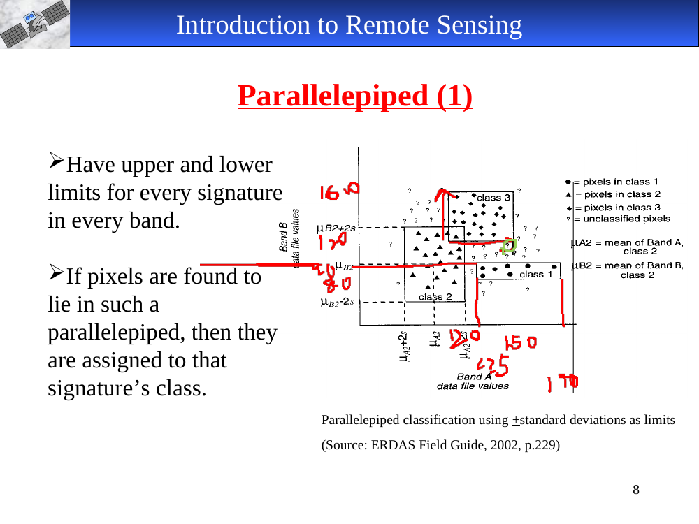
Diagram uses ±1 standard deviation as the limits. Source: ERDAS Field Guide 2002 p. 229.
Parallelepiped (1) — concept.
- For each signature, define an upper and lower limit in every band.
- Pixels whose values fall inside the resulting n-dimensional box are assigned to that signature’s class.
- Diagram uses ±1 std dev as the limits (ERDAS Field Guide 2002 p. 229).
Parallelepiped (2) — pros and cons
Limits can be any values — min/max of training data, ±σ, or user-supplied based on knowledge.
Advantages
- Very simple and fast supervised classifier.
- Useful for a first-pass broad classification.
Disadvantages
- Gap regions — pixels outside all boxes stay unclassified.
- Corner overlaps — pixels in overlapping corners may be classified improperly.
Parallelepiped (2) — when to use it.
- Limits can be anything the user specifies — e.g., min/max of training data, or ±1 or ±2 σ.
- Advantages:
- Very simple, very fast.
- Good as a first-pass broad classification.
- Disadvantages:
- Gap regions (pixels outside all boxes) stay unclassified.
- Corners where boxes overlap may be assigned incorrectly.
Minimum Distance (1)
Computes the spectral distance between the candidate pixel's measurement vector V and the mean vector Bm for each class signature:
A pixel belongs to class m if the spectral distance to that class is the smallest.
Source: ERDAS Field Guide 2002 p. 232.
Minimum Distance (1) — the formula.
For a pixel with measurement vector V and class m mean vector B_m:
\[D_{\text{ist}}(\text{class}_m) \;=\; \sqrt{\sum_{k=1}^{n} (B_{m,k} - V_k)^2}\]- Euclidean distance across all n bands.
- The pixel is assigned to the class whose distance is smallest (closest mean).
Source: ERDAS Field Guide 2002 p. 232.
Minimum Distance (2) — pros and cons
Advantages
- No unclassified pixels.
- A fast decision rule.
Disadvantages
- Pixels that should be unclassified — because they're not spectrally close to any sample mean — will be "force-fit" into the nearest class anyway.
- Does not consider class variability (a tight class and a wide class are treated equally).
Minimum Distance (2) — advantages and disadvantages.
Advantages: - No unclassified pixels (every pixel has a nearest mean). - Fast decision rule.
Disadvantages: - Pixels that should be unclassified — because they’re not close to any training class — will still be assigned somewhere (a “force-fit”). - Does not consider class variability (two classes with very different spreads are treated equally).
Maximum Likelihood (1)
Based on the probability that a pixel belongs to a particular class:
A pixel at x is assigned to class c if the likelihood that the correct class is c is the largest.
Source: ERDAS IMAGINE v8.3 Professional Training Reference Manual 1997 p. 29.
Maximum Likelihood (1) — the probability idea.
A pixel belongs to a class if the probability of membership in that class is highest:
\[p_c > p_i \quad \text{for all } i = 1, 2, 3, \ldots, m\ \text{classes}\]- The pixel at x is assigned to class c if the likelihood that the correct class is c is the largest.
- Reference: ERDAS Imagine v8.3 Professional Training Reference Manual (1997) p. 29.
Maximum likelihood — formal statement
Assumption: data for each class is normally distributed.
- Let C = (C₁, C₂, …, Cnc) be the set of nc classes.
- For a pixel with gray-level vector x, the posterior probability that x belongs to class Ci is
P(Ci | x). - x is assigned to class Ci if
P(Ci | x) ≥ P(Cj | x)for all j ≠ i.
Reference: Gong lecture notes, UC Berkeley.
Maximum Likelihood — formal statement.
- Assumption: data for each class is normally distributed (Gaussian) in feature space.
- Let C = (C₁, C₂, …, C_nc) be the set of nc classes.
- For a pixel with gray-level vector x, compute posterior probability P(Cᵢ | x) for every class.
- Assign the pixel to Cᵢ if
P(Cᵢ | x) ≥ P(Cⱼ | x)for all j ≠ i — i.e., the class with the highest posterior wins. - Reference: Gong lecture notes, UC Berkeley (nature.berkeley.edu).
Maximum Likelihood (2) — when it applies
The most common supervised decision rule.
Assumptions:
- Probabilities are equal for all classes.
- The input bands have normal distributions — training-data statistics for each class in each band are normally distributed.
Maximum Likelihood (2) — when it applies.
- The most commonly used decision rule in supervised classification.
- Assumptions:
- Prior probabilities are equal for all classes (drop this → Bayesian rule, slide 15).
- Each input band has a normal distribution inside each class.
- Works well when classes are well-sampled and spectrally distinct; struggles on rare classes or non-Gaussian distributions.
Maximum Likelihood / Bayesian (3)
Bayesian decision rule — if the user has prior knowledge that the probabilities are not equal for all classes, they can specify weight factors per class. This variation of Max Likelihood is called the Bayesian decision rule (Hord 1982).
Characteristics:
- The most accurate classifier (when assumptions hold).
- Takes the most variables into account.
- If band histograms are not normally distributed, Parallelepiped or Min Distance may actually give better results.
Maximum Likelihood / Bayesian (3).
- Bayesian variant — if the user has prior knowledge that class probabilities are NOT equal, they can specify weight factors per class.
- Reference: Hord 1982.
Characteristics: - The most accurate classifier of the four, when assumptions hold. - Takes the most variables into account (means, covariances, priors). - But: if the bands are not normally distributed, Parallelepiped or Min Distance may actually give better results.
Maximum Likelihood / Bayesian (4) — full rule
The pixel is assigned to the class for which D is the lowest:
- X — measurement vector of the candidate pixel.
- Mc — mean vector of the data in class c.
- Vc — covariance matrix of the data in class c.
- |Vc| — determinant of Vc.
- Vc−1 — inverse of Vc.
- T — transposition.
- ac — probability that class c occurs in the image (equal for all classes, or entered from a priori knowledge).
The last term (X − Mc)T Vc−1 (X − Mc) is the squared Mahalanobis distance — distance from the pixel to the class mean, scaled by the class's covariance. Mahalanobis alone (without the log-determinant and log-prior terms) is its own decision rule.
Maximum Likelihood / Bayesian (4) — full decision rule.
The pixel is assigned to the class for which D is the lowest:
\[D \;=\; \log_e(a_c) \;-\; \tfrac{1}{2}\log_e(|V_c|) \;-\; \tfrac{1}{2}(X - M_c)^{\!T}\,V_c^{-1}(X - M_c)\]- X — measurement vector of the candidate pixel.
- M_c — mean vector of the data in class c.
- V_c — covariance matrix of class c.
-
** V_c ** — determinant of V_c. - V_c⁻¹ — inverse of V_c.
- T — transposition.
-
a_c — prior probability that class c occurs in the image (equal for all classes, or user-entered from a priori knowledge).
- The third term is the Mahalanobis distance squared — distance from the pixel to the class mean, scaled by the class’s covariance. Mahalanobis alone (without the first two log terms) is its own decision rule.
Deck: Ma_RS9-SupervisedClassification2026.ppt — 16 slides.
Download original
·
Edit our reproduction